Linux context switches per second

Context Switch Definition

A context switch (also sometimes referred to as a process switch or a task switch) is the switching of the CPU (central processing unit) from one process or thread to another.

A process (also sometimes referred to as a task) is an executing (i.e., running) instance of a program. In Linux, threads are lightweight processes that can run in parallel and share an address space (i.e., a range of memory locations) and other resources with their parent processes (i.e., the processes that created them).

A context is the contents of a CPU’s registers and program counter at any point in time. A register is a small amount of very fast memory inside of a CPU (as opposed to the slower RAM main memory outside of the CPU) that is used to speed the execution of computer programs by providing quick access to commonly used values, generally those in the midst of a calculation. A program counter is a specialized register that indicates the position of the CPU in its instruction sequence and which holds either the address of the instruction being executed or the address of the next instruction to be executed, depending on the specific system.

Context switching can be described in slightly more detail as the kernel (i.e., the core of the operating system) performing the following activities with regard to processes (including threads) on the CPU: (1) suspending the progression of one process and storing the CPU’s state (i.e., the context) for that process somewhere in memory, (2) retrieving the context of the next process from memory and restoring it in the CPU’s registers and (3) returning to the location indicated by the program counter (i.e., returning to the line of code at which the process was interrupted) in order to resume the process.

A context switch is sometimes described as the kernel suspending execution of one process on the CPU and resuming execution of some other process that had previously been suspended. Although this wording can help clarify the concept, it can be confusing in itself because a process is, by definition, an executing instance of a program. Thus the wording suspending progression of a process might be preferable.

Context Switches and Mode Switches

Context switches can occur only in kernel mode. Kernel mode is a privileged mode of the CPU in which only the kernel runs and which provides access to all memory locations and all other system resources. Other programs, including applications, initially operate in user mode, but they can run portions of the kernel code via system calls. A system call is a request in a Unix-like operating system by an active process (i.e., a process currently progressing in the CPU) for a service performed by the kernel, such as input/output (I/O) or process creation (i.e., creation of a new process). I/O can be defined as any movement of information to or from the combination of the CPU and main memory (i.e. RAM), that is, communication between this combination and the computer’s users (e.g., via the keyboard or mouse), its storage devices (e.g., disk or tape drives), or other computers.

The existence of these two modes in Unix-like operating systems means that a similar, but simpler, operation is necessary when a system call causes the CPU to shift to kernel mode. This is referred to as a mode switch rather than a context switch, because it does not change the current process.

Context switching is an essential feature of multitasking operating systems. A multitasking operating system is one in which multiple processes execute on a single CPU seemingly simultaneously and without interfering with each other. This illusion of concurrency is achieved by means of context switches that are occurring in rapid succession (tens or hundreds of times per second). These context switches occur as a result of processes voluntarily relinquishing their time in the CPU or as a result of the scheduler making the switch when a process has used up its CPU time slice.

A context switch can also occur as a result of a hardware interrupt, which is a signal from a hardware device (such as a keyboard, mouse, modem or system clock) to the kernel that an event (e.g., a key press, mouse movement or arrival of data from a network connection) has occurred.

Intel 80386 and higher CPUs contain hardware support for context switches. However, most modern operating systems perform software context switching, which can be used on any CPU, rather than hardware context switching in an attempt to obtain improved performance. Software context switching was first implemented in Linux for Intel-compatible processors with the 2.4 kernel.

One major advantage claimed for software context switching is that, whereas the hardware mechanism saves almost all of the CPU state, software can be more selective and save only that portion that actually needs to be saved and reloaded. However, there is some question as to how important this really is in increasing the efficiency of context switching. Its advocates also claim that software context switching allows for the possibility of improving the switching code, thereby further enhancing efficiency, and that it permits better control over the validity of the data that is being loaded.

The Cost of Context Switching

Context switching is generally computationally intensive. That is, it requires considerable processor time, which can be on the order of nanoseconds for each of the tens or hundreds of switches per second. Thus, context switching represents a substantial cost to the system in terms of CPU time and can, in fact, be the most costly operation on an operating system.

Consequently, a major focus in the design of operating systems has been to avoid unnecessary context switching to the extent possible. However, this has not been easy to accomplish in practice. In fact, although the cost of context switching has been declining when measured in terms of the absolute amount of CPU time consumed, this appears to be due mainly to increases in CPU clock speeds rather than to improvements in the efficiency of context switching itself.

One of the many advantages claimed for Linux as compared with other operating systems, including some other Unix-like systems, is its extremely low cost of context switching and mode switching.

Created October 25, 2004. Updated May 28, 2006.
Copyright © 2004 — 2006 The Linux Information Project. All Rights Reserved.

Источник

Measuring context switching and memory overheads for Linux threads

In this post I want to explore the costs of threads on modern Linux machines, both in terms of time and space. The background context is designing high-load concurrent servers, where using threads is one of the common schemes.

Important disclaimer: it’s not my goal here to provide an opinion in the threads vs. event-driven models debate. Ultimately, both are tools that work well in some scenarios and less well in others. That said, one of the major criticisms of a thread-based model is the cost — comments like «but context switches are expensive!» or «but a thousand threads will eat up all your RAM!», and I do intend to study the data underlying such claims in more detail here. I’ll do this by presenting multiple code samples and programs that make it easy to explore and experiment with these measurements.

Linux threads and NPTL

In the dark, old ages before version 2.6, the Linux kernel didn’t have much specific support for threads, and they were more-or-less hacked on top of process support. Before futexes there was no dedicated low-latency synchronization solution (it was done using signals); neither was there much good use of the capabilities of multi-core systems [1].

The Native POSIX Thread Library (NPTL) was proposed by Ulrich Drepper and Ingo Molnar from Red Hat, and integrated into the kernel in version 2.6, circa 2005. I warmly recommend reading its design paper. With NPTL, thread creation time became about 7x faster, and synchronization became much faster as well due to the use of futexes. Threads and processes became more lightweight, with strong emphasis on making good use of multi-core processors. This roughly coincided with a much more efficient scheduler, which made juggling many threads in the Linux kernel even more efficient.

Even though all of this happened 13 years ago, the spirit of NPTL is still easily observable in some system programming code. For example, many thread and synchronization-related paths in glibc have nptl in their name.

Threads, processes and the clone system call

This was originally meant to be a part of this larger article, but it was getting too long so I split off a separate post on launching Linux processes and threads with clone, where you can learn about the clone system call and some measurements of how expensive it is to launch new processes and threads.

The rest of this post will assume this is familiar information and will focus on context switching and memory usage.

What happens in a context switch?

In the Linux kernel, this question has two important parts:

1. When does a kernel switch happen
2. How it happens

The following deals mostly with (2), assuming the kernel has already decided to switch to a different user thread (for example because the currently running thread went to sleep waiting for I/O).

The first thing that happens during a context switch is a switch to kernel mode, either through an explicit system call (such as write to some file or pipe) or a timer interrupt (when the kernel preempts a user thread whose time slice has expired). This requires saving the user space thread’s registers and jumping into kernel code.

Next, the scheduler kicks in to figure out which thread should run next. When we know which thread runs next, there’s the important bookkeeping of virtual memory to take care of; the page tables of the new thread have to be loaded into memory, etc.

Finally, the kernel restores the new thread’s registers and cedes control back to user space.

All of this takes time, but how much time, exactly? I encourage you to read some additional online resources that deal with this question, and try to run benchmarks like lm_bench; what follows is my attempt to quantify thread switching time.

How expensive are context switches?

To measure how long it takes to switch between two threads, we need a benchmark that deliberatly triggers a context switch and avoids doing too much work in addition to that. This would be measuring just the direct cost of the switch, when in reality there is another cost — the indirect one, which could even be larger. Every thread has some working set of memory, all or some of which is in the cache; when we switch to another thread, all this cache data becomes unneeded and is slowly flushed out, replaced by the new thread’s data. Frequent switches back and forth between the two threads will cause a lot of such thrashing.

In my benchmarks I am not measuring this indirect cost, because it’s pretty difficult to avoid in any form of multi-tasking. Even if we «switch» between different asynchronous event handlers within the same thread, they will likely have different memory working sets and will interfere with each other’s cache usage if those sets are large enough. I strongly recommend watching this talk on fibers where a Google engineer explains their measurement methodology and also how to avoid too much indirect switch costs by making sure closely related tasks run with temporal locality.

These code samples measure context switching overheads using two different techniques:

1. A pipe which is used by two threads to ping-pong a tiny amount of data. Every read on the pipe blocks the reading thread, and the kernel switches to the writing thread, and so on.
2. A condition variable used by two threads to signal an event to each other.

There are additional factors context switching time depends on; for example, on a multi-core CPU, the kernel can occasionally migrate a thread between cores because the core a thread has been previously using is occupied. While this helps utilize more cores, such switches cost more than staying on the same core (again, due to cache effects). Benchmarks can try to restrict this by running with taskset pinning affinity to one core, but it’s important to keep in mind this only models a lower bound.

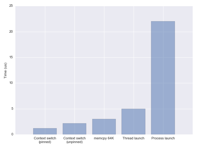
Using the two techniques I’m getting fairly similar results: somewhere between 1.2 and 1.5 microseconds per context switch, accounting only for the direct cost, and pinning to a single core to avoid migration costs. Without pinning, the switch time goes up to

2.2 microseconds [2]. These numbers are largely consistent with the reports in the fibers talk mentioned above, and also with other benchmarks found online (like lat_ctx from lmbench).

What does this mean in practice?

So we have the numbers now, but what do they mean? Is 1-2 us a long time? As I have mentioned in the post on launch overheads, a good comparison is memcpy, which takes 3 us for 64 KiB on the same machine. In other words, a context switch is a bit quicker than copying 64 KiB of memory from one location to another.

1-2 us is not a long time by any measure, except when you’re really trying to optimize for extremely low latencies or high loads.

As an example of an artificially high load, here is another benchmark which writes a short message into a pipe and expects to read it from another pipe. On the other end of the two pipes is a thread that echoes one into the other.

Running the benchmark on the same machine I used to measure the context switch times, I get

400,000 iterations per second (this is with taskset to pin to a single core). This makes perfect sense given the earlier measurements, because each iteration of this test performs two context switches, and at 1.2 us per switch this is 2.4 us per iteration.

You could claim that the two threads compete for the same CPU, but if I don’t pin the benchmark to a single core, the number of iterations per second halves. This is because the vast majority of time in this benchmark is spent in the kernel switching from one thread to the other, and the core migrations that occur when it’s not pinned greatly ouweigh the loss of (the very minimal) parallelism.

Just for fun, I rewrote the same benchmark in Go; two goroutines ping-ponging short message between themselves over a channel. The throughput this achieves is dramatically higher — around 2.8 million iterations per second, which leads to an estimate of

170 ns switching between goroutines [3]. Since switching between goroutines doesn’t require an actual kernel context switch (or even a system call), this isn’t too surprising. For comparison, Google’s fibers use a new Linux system call that can switch between two tasks in about the same time, including the kernel time.

A word of caution: benchmarks tend to be taken too seriously. Please take this one only for what it demonstrates — a largely synthetical workload used to poke into the cost of some fundamental concurrency primitives.

Remember — it’s quite unlikely that the actual workload of your task will be negligible compared to the 1-2 us context switch; as we’ve seen, even a modest memcpy takes longer. Any sort of server logic such as parsing headers, updating state, etc. is likely to take orders of magnitude longer. If there’s one takeaway to remember from these sections is that context switching on modern Linux systems is super fast.

Memory usage of threads

Now it’s time to discuss the other overhead of a large number of threads — memory. Even though all threads in a process share their, there are still areas of memory that aren’t shared. In the post about clone we’ve mentioned page tables in the kernel, but these are comparatively small. A much larger memory area that it private to each thread is the stack.

The default per-thread stack size on Linux is usually 8 MiB, and we can check what it is by invoking ulimit:

To see this in action, let’s start a large number of threads and observe the process’s memory usage. This sample launches 10,000 threads and sleeps for a bit to let us observe its memory usage with external tools. Using tools like top (or preferably htop) we see that the process uses

80 GiB of virtual memory, with about 80 MiB of resident memory. What is the difference, and how can it use 80 GiB of memory on a machine that only has 16 available?

Virtual vs. Resident memory

A short interlude on what virtual memory means. When a Linux program allocates memory (with malloc) or otherwise, this memory initially doesn’t really exist — it’s just an entry in a table the OS keeps. Only when the program actually accesses the memory is the backing RAM for it found; this is what virtual memory is all about.

Therefore, the «memory usage» of a process can mean two things — how much virtual memory it uses overall, and how much actual memory it uses. While the former can grow almost without bounds — the latter is obviously limited to the system’s RAM capacity (with swapping to disk being the other mechanism of virtual memory to assist here if usage grows above the side of physical memory). The actual physical memory on Linux is called «resident» memory, because it’s actually resident in RAM.

There’s a good StackOverflow discussion of this topic; here I’ll just limit myself to a simple example:

This program starts by allocating 400 MiB of memory (assuming an int size of 4) with malloc, and later «touches» this memory by writing a number into every element of the allocated array. It reports its own memory usage at every step — see the full code sample for the reporting code [4]. Here’s the output from a sample run:

The most interesting thing to note is how vm size remains the same between the second and third steps, while max RSS grows from the initial value to 400 MiB. This is precisely because until we touch the memory, it’s fully «virtual» and isn’t actually counted for the process’s RAM usage.

Therefore, distinguishing between virtual memory and RSS in realistic usage is very important — this is why the thread launching sample from the previous section could «allocate» 80 GiB of virtual memory while having only 80 MiB of resident memory.

Back to memory overhead for threads

As we’ve seen, a new thread on Linux is created with 8 MiB of stack space, but this is virtual memory until the thread actually uses it. If the thread actually uses its stack, resident memory usage goes up dramatically for a large number of threads. I’ve added a configuration option to the sample program that launches a large number of threads; with it enabled, the thread function actually uses stack memory and from the RSS report it is easy to observe the effects. Curiously, if I make each of 10,000 threads use 400 KiB of memory, the total RSS is not 4 GiB but around 2.6 GiB [5].

How to we control the stack size of threads? One option is using the ulimit command, but a better option is with the pthread_attr_setstacksize API. The latter is invoked programatically and populates a pthread_attr_t structure that’s passed to thread creation. The more interesting question is — what should the stack size be set to?

As we have seen above, just creating a large stack for a thread doesn’t automatically eat up all the machine’s memory — not before the stack is being used. If our threads actually use large amounts of stack memory, this is a problem, because this severely limits the number of threads we can run concurrently. Note that this is not really a problem with threads — but with concurrency; if our program uses some event-driven approach to concurrency and each handler uses a large amount of memory, we’d still have the same problem.

If the task doesn’t actually use a lot of memory, what should we set the stack size to? Small stacks keep the OS safe — a deviant program may get into an infinite recursion and a small stack will make sure it’s killed early. Moreover, virtual memory is large but not unlimited; especially on 32-bit OSes, we might not have 80 GiB of virtual address space for the process, so a 8 MiB stack for 10,000 threads makes no sense. There’s a tradeoff here, and the default chosen by 32-bit Linux is 2 MiB; the maximal virtual address space available is 3 GiB, so this imposes a limit of

1500 threads with the default settings. On 64-bit Linux the virtual address space is vastly larger, so this limitation is less serious (though other limits kick in — on my machine the maximal number of threads the OS lets one process start is about 32K).

Therefore I think it’s more important to focus on how much actual memory each concurrent task is using than on the OS stack size limit, as the latter is simply a safety measure.

Conclusion

The numbers reported here paint an interesting picture on the state of Linux multi-threaded performance in 2018. I would say that the limits still exist — running a million threads is probably not going to make sense; however, the limits have definitely shifted since the past, and a lot of folklore from the early 2000s doesn’t apply today. On a beefy multi-core machine with lots of RAM we can easily run 10,000 threads in a single process today, in production. As I’ve mentioned above, it’s highly recommended to watch Google’s talk on fibers; through careful tuning of the kernel (and setting smaller default stacks) Google is able to run an order of magnitude more threads in parallel.

Whether this is sufficient concurrency for your application is very obviously project-specific, but I’d say that for higher concurrencies you’d probably want to mix in some asynchronous processing. If 10,000 threads can provide sufficient concurrency — you’re in luck, as this is a much simpler model — all the code within the threads is serial, there are no issues with blocking, etc.

Источник