Resident set size linux

Что такое RSS и VSZ в управлении памятью Linux

Что такое RSS и VSZ в управлении памятью Linux? В многопоточной среде, как можно управлять и отслеживать обе эти функции?

RSS — это размер резидентного набора и используется, чтобы показать, сколько памяти выделено этому процессу и находится в оперативной памяти. Он не включает память, которая выгружается. Он включает память из общих библиотек, пока страницы из этих библиотек фактически находятся в памяти. Он включает в себя всю память стека и кучи.

VSZ — это размер виртуальной памяти. Он включает в себя всю память, к которой может обращаться процесс, включая память, которая выгружается, память, которая выделена, но не используется, и память из общих библиотек.

Таким образом, если процесс A имеет двоичный файл размером 500 КБ и связан с 2500 КБ совместно используемых библиотек, имеет 200 КБ выделенных стеков / кучи, из которых 100 КБ фактически находится в памяти (остальная часть поменялась местами или не используется), и он фактически загрузил только 1000 КБ совместно используемых библиотек. и 400K своего двоичного файла:

Поскольку часть памяти является общей, многие процессы могут использовать ее, поэтому, если вы сложите все значения RSS, вы легко сможете получить больше места, чем в вашей системе.

Память, которая выделяется, также может отсутствовать в RSS, пока она не будет фактически использована программой. Поэтому, если ваша программа выделяет кучу памяти заранее, а затем использует ее со временем, вы можете увидеть, что RSS растет, а VSZ остается прежним.

Существует также PSS (пропорциональный размер набора). Это более новая мера, которая отслеживает общую память как пропорцию, используемую текущим процессом. Так что, если раньше было два процесса, использующих одну и ту же общую библиотеку:

Все потоки имеют одинаковое адресное пространство, поэтому RSS, VSZ и PSS для каждого потока идентичны всем другим потокам в процессе. Используйте ps или top для просмотра этой информации в linux / unix.

Существует гораздо больше, чем это, чтобы узнать больше, проверьте следующие ссылки:

Источник

Требуется объяснение размера резидентного набора / виртуального размера

Я обнаружил, что pidstat это будет хорошим инструментом для мониторинга процессов. Я хочу рассчитать среднее использование памяти для определенного процесса. Вот пример выходных данных:

(Это часть вывода из pidstat -r -p 7276 .)

Должен ли я использовать информацию о резидентном наборе (RSS) или виртуальном размере (VSZ) для расчета среднего потребления памяти? Я прочитал кое-что в Википедии и на форумах, но я не уверен, что полностью понимаю различия. Кроме того, кажется, что ни один из них не является надежным. Итак, как я могу контролировать процесс, чтобы получить его использование памяти?

Любая помощь по этому вопросу будет полезна.

RSS — это количество памяти, которое этот процесс в настоящее время имеет в основной памяти (RAM). VSZ — это количество виртуальной памяти, которое имеет процесс в целом. Это включает в себя все типы памяти, как в оперативной памяти, так и подкачки. Эти числа могут быть искажены, потому что они также включают в себя общие библиотеки и другие типы памяти. У вас может быть пятьсот экземпляров bash , и общий размер их памяти не будет суммой их значений RSS или VSZ.

Если вам необходимо получить более подробное представление об объеме памяти процесса, у вас есть несколько вариантов. Вы можете пройти /proc/$PID/map и отсеять то, что вам не нравится. Если это общие библиотеки, расчет может быть сложным в зависимости от ваших потребностей (что, я думаю, я помню).

Если вас волнует только размер кучи процесса, вы всегда можете просто проанализировать [heap] запись в map файле. Размер, выделенный ядром для кучи процесса, может отражать или не отражать точное количество байтов, которые процесс запросил для выделения. Есть мелкие детали, внутренности ядра и оптимизации, которые могут скинуть это. В идеальном мире это будет столько, сколько нужно вашему процессу, округленное до ближайшего кратного размера системной страницы ( getconf PAGESIZE скажет вам, что это такое — на ПК это, вероятно, 4096 байт).

Если вы хотите увидеть, сколько памяти выделил процесс , одним из лучших способов является отказ от метрик на стороне ядра. Вместо этого вы используете LD_PRELOAD механизм выделения (удаления) памяти кучи библиотеки C с помощью этого механизма. Лично я немного ругаюсь, valgrind чтобы получить информацию об этом. (Обратите внимание, что применение инструментов потребует перезапуска процесса.)

Обратите внимание: поскольку вы также можете тестировать время выполнения, это valgrind сделает ваши программы немного медленнее (но, вероятно, в пределах ваших допусков).

Источник

UNIX: top и ps — VIRT, RES, SHR и SWAP память

VIRT (Virtual memory) — отображает общий объём памяти, который может использоваться процессом в данный момент. Включает в себя реально используемую память, другую память (например — память видеокарты), файлы на диске, загруженные в память (например — файлы библиотек), и память, совместно используемую с другими процессами ( SHR или Shared memory ). Она же отображается как VSZ в результатах ps (Process status) .

RES (Resident memory size) — отображает, сколько физической памяти занято процессом (используется для отображения в колонке %MEM в top -е). Она же отображается как RSS в результатах ps (Process status) .

SHR (Shared Memory size) — отображает объём VIRT памяти, который используется процессом совместно с другими процессами, например — файлы библиотек.

SWAP (Swapped size) — память, которая в данный момент не используется (не- RES ), но доступна процессу, при этом она «выгружена» в swap -раздел диска.

o: VIRT — Virtual Image (kb)
The total amount of virtual memory used by the task. It includes all code, data and shared libraries plus pages that have been swapped out. (Note: you can define the STATSIZE=1 environment variable and
the VIRT will be calculated from the /proc/#/state VmSize field.)

p: SWAP — Swapped size (kb)
Per-process swap values are now taken from /proc/#/status VmSwap field.

q: RES — Resident size (kb)
The non-swapped physical memory a task has used.

VSZ (VSS) — Virtual Size in Kbytes (alias vsize) или Virtual memory — особый уровень абстракции «над» архитектурой физической памяти.

Каждый процесс получает в использование виртуальное адресное пространство, и при обращении к адресу в нём — адрес сначала конвертируется в адрес физической памяти (main memory — MM , она же RAM) при помощи Memory Management Unit (MMU) . Данные в виртуальном адресном пространстве могут располагаться в основной памяти, на диске (в swap -файле), сразу в обоих местах или на какой-то внешней памяти (например — памяти видеокарты). Однако, как только процесс запрашивает какие-то данные, которые в настоящий момент не находятся в основной памяти системы — они туда загружаются. Таким образом, процесс не считывает данные напрямую с диска ( memory mapping ), но некоторые или все его ресурсы могут находится на «внешней памяти» в любое время, а его страницы памяти могут быть выгружены в swap, что бы освободить память для других процессов.

RSS — Resident Set Size — количество выеделенной процессу физической ( MM ) памяти в настоящий момент. Это физическая память, которая используется для рамзмещения страниц виртуальной памяти ( virtual memory pages ), которая используется процессом постоянно. RSS всегда будет менее или равна памяти VSZ.

Вообще это очень большая тема, потому — несколько ссылок:

Источник

Working Set Size Estimation

The Working Set Size (WSS) is how much memory an application needs to keep working. Your application may have 100 Gbytes of main memory allocated and page mapped, but it is only touching 50 Mbytes each second to do its job. That’s the working set size: the «hot» memory that is frequently used. It is useful to know for capacity planning and scalability analysis.

You may never have seen WSS measured by any tool (when I created this page, I hadn’t either). OSes usually show you these metrics:

• Virtual memory: Not real memory. It’s an artifact of a virtual memory system. For on-demand memory systems like Linux, malloc() immediately returns virtual memory, which is only promoted to real memory later when used (promoted via a page fault).
• Resident memory or Resident set size (RSS): Main memory. Real memory pages that are currently mapped.
• Proportional set size (PSS): RSS with shared memory divided among users.

These are easily tracked by the kernel as it manages virtual and main memory allocation. But when your application is in user-mode doing load and store instructions across its WSS, the kernel isn’t (usually) involved. So there’s no obvious way a kernel can provide a WSS metric.

On this page I’ll summarize WSS objectives and different approaches for WSS estimation, applicable to any OS. This includes my wss tools for Linux, which do page-based WSS estimation by use of referenced and idle page flags, and my WSS profile charts.

Table of contents:

Objectives

What you intend to use WSS for will direct how you measure it. Consider these three scenarios:

A) You are sizing main memory for an application, with the intent to keep it from paging (swapping). WSS will be measured in bytes over a long interval, say, one minute.

B) You are optimizing CPU caches. WSS will be measured in unique cachelines accessed over a short interval, say, one second or less. The cacheline size is architecture dependent, usually 64 bytes.

C) You are optimizing the TLB caches (translation lookaside buffer: a memory management unit cache for virtual to physical translation). WSS will be measured in unique pages accessed over a short interval, say, one second or less. The pagesize is architecture and OS configuration dependent, 4 Kbytes is commonly used.

You can figure out the cacheline size on Linux using cpuid, and the page size using pmap -XX.

1. Estimation

You can try estimating it: how much memory would your application touch to service a request, or over a short time interval? If you have access to the developer of the application, they may already have a reasonable idea. Depending on your objective, you’ll need to ask either how many unique bytes, cachelines, or pages would be referenced.

2. Observation: Paging/Swapping Metrics

Paging metrics are commonly available across different operating systems. Linux, BSD, and other Unixes print them in vmstat, OS X in vm_stat. There are usually also scanning metrics, showing that the system is running low on memory and is spending more time keeping free lists populated.

The basic idea with these metrics is:

• Sustained paging/swapping == WSS is larger than main memory.
• No paging/swapping, but sustained scanning == WSS is close to main memory size.
• No paging/swapping or scanning == WSS is lower than main memory size.

What’s interesting about sustained paging, as opposed to other memory counters (like resident memory aka RSS: resident set size, virtual memory, Linux «active»/»inactive» memory, etc), is that the sustained page-ins tell us that the application is actually using that memory to do its job. With counters like resident set size (RSS), you don’t know how much of that the application is actually using each second.

On Linux, this requires a swap device to be configured as the target for paging, which on many systems is not the case. Without a swap device, the Linux out-of-memory (OOM) killer can kill sacrificial processes to free space, which doesn’t tell us a great deal about WSS.

2.1. Paging/Swapping

Finding paging/swapping counters is usually easy. Here they are on Linux (output columns don’t line up with the header):

Linux calls paging «swapping» (in other Unixes, swapping refers to moving entire threads to the swap device, and paging refers to just the pages). The above example shows no swapping is active.

2.2. Scanning

Older Unixes used a page scanner to search all memory for not-recently-used pages for paging out, and reported a scan rate in vmstat. The scan rate was only non-zero when the system was running out of memory, and increased based on demand. That scan rate could be used as an early warning that the system was about to run out of main memory (if it wasn’t paging already), and the rate as the magnitude. Note that it needs to be sustained scanning (eg, 30 seconds) to give an indication about WSS. An application could allocate and populate memory that was scanned and paged out, but then not used again, causing a burst in scanning and paging. That’s cold memory: it’s not WSS. WSS is active, and if paged out will be quickly paged back in again, causing paging churn: sustained scanning and paging.

Linux maintains «active» and «inactive» lists of memory, so that eligible pages can be found quickly by walking the inactive list. At various points in time, pages will be moved from an active list to an inactive list, where they have a chance to be «reclaimed» and moved back to active, before swapped out when needed. Active/inactive memory sizes are available in /proc/meminfo. To check if the system is getting close to the swapping point, the vmscan tracepouints can be used. Eg:

You could choose just the vmscan:mm_vmscan_kswapd_wake tracepoint as a low-overhead (because it is low frequency) indicator. Measuring it per-second:

You may also see kswapd show up in process monitors, consuming %CPU.

3. Experimentation: Main Memory Shrinking

Worth mentioning but not recommended: I saw this approach used many years ago on Unix systems where paging was more commonly configured and used, and one could experimentally reduce the memory available to a running application while watching how heavily it was paging. There’d be a point where the application was generally «happy» (low paging), and then where it wasn’t (suddenly high paging). That point is a measure of WSS.

4. Observation: PMCs

Performance Monitoring Counters (PMCs) can provide some clues to your WSS, and can be measured on Linux using perf. Here’s a couple of workloads, measured using my pmcarch tool from pmc-cloud-tools:

Workload A has a Last Level Cache (LLC, aka L3) hit ratio of over 99.8%. Might its WSS be smaller than the LLC size? Probably. The LLC size is 24 Mbytes (the CPU is: Intel(R) Xeon(R) Platinum 8124M CPU @ 3.00GHz). This is a synthetic workload with a uniform access distribution, where I know the WSS is 10 Mbytes.

Workload B has a LLC hit ratio of 39%. Not really fitting at all. It’s also synthetic and uniform, with a WSS of 100 Mbytes, bigger than the LLC. So that makes sense.

With a 61% LLC hit ratio, you might guess it is somewhere in-between workload A (10 Mbytes) and B (100 Mbytes). But no, this is also 100 Mbytes. I elevated its LLC hit ratio by making the access pattern non-uniform. What can we do about that? There are a lot of PMCs: for caches, the MMU and TLB, and memory events, so I think it’s possible that we could model a CPU, plug in all these numbers, and have it estimate not just the WSS but also the access pattern. I haven’t seen anyone try this (surely someone has), so I don’t have any reference about it. It’s been on my todo list to try for a while. It also involves truly understanding each PMC: they often have measurement caveats.

Here’s a screenshot of cpucache, a new tool I just added to pmc-cloud-tools, which shows some of these additional PMCs:

Note that CPU caches usually operate on cachelines (eg, 64 bytes), so a workload of random 1 byte reads becomes 64 byte reads, inflating the WSS. Although, if I’m analyzing CPU cache scalability, I want to know the WSS in terms of cachelines anyway, as that’s what will be cached.

At the very least, PMCs can tell you this:

100% hit ratio and a high ref count, then a single-threaded cacheline-based WSS is smaller than that cache, and might be bigger than any before it.

If the L2 was 8 Mbytes, the LLC was 24 Mbytes, and the LLC had a

100% hit ratio and a high reference count, you might conclude that the WSS is between 8 and 24 Mbytes. If it was smaller than 8 Mbytes, then it would fit in the L2, and the LLC would no longer have a high reference count. I said «might be» because a smaller workload might not cache in the L2 for other reasons: eg, set associativity.

I also had to qualify this as single-threaded. What’s wrong with multi-threaded? Consider a multi-core multi-socket server running a multi-threaded application, where each thread has effectively its own working set it is operating on. The application’s combined working set size can be cached by multiple CPU caches: multiple L1, L2, and LLCs. It may have a

100% LLC hit ratio, but the WSS is bigger than a single LLC, because it is living in more than one.

5. Experimentation: CPU Cache Flushing

Just an idea. I couldn’t find an example of anyone doing it, but for CPU caches I imagine cache flushing combined with PMCs can be used for WSS estimation. Flush the cache, then measure how quickly it takes for the LLC to fill and begin evicting again. The slower it takes, the smaller the WSS (probably). There’s usually CPU instructions to help with cache flushing, provided they are enabled:

There’s also other caches this approach can be applied to. The MMU TLB can be flushed (at least, the kernel knows how). The Linux file system cache can be flushed with /proc/sys/vm/drop_caches, and then growth tracked over time via OS metrics (eg, free).

6. Experimentation: PTE Accessed Bit

These approaches make use of a page table entry (PTE) «Accessed» bit, which is normally updated by the CPU MMU as it accesses memory pages, and can be read and cleared by the kernel. This can be used to provide a page-based WSS estimation by clearing the accessed bit on all of a process’s pages, waiting an interval, and then checking how many pages the bit returned to. It has the advantage of no extra overhead when the accessed bit is updated, as the MMU does it anyway.

6.1. Linux Reference Page Flag

This uses a kernel feature added in Linux 2.6.22: the ability to set and read the referenced page flag from user space, added for analyzing memory usage. The referenced page flag is really the PTE accessed bit (_PAGE_BIT_ACCESSED in Linux). I developed wss.pl as a front-end to this feature. The following uses it on a MySQL database server (mysqld), PID 423, and measures its working set size for 0.1 seconds (100 milliseconds):

In 100 ms, mysqld touched 28 Mbytes worth of pages, out of its 404 Mbytes of total main memory. Why did I use a 100 ms interval? Short durations can be useful for understanding how well a WSS will fit into the CPU caches (L1/L2/L3, TLB L1/L2, etc). In this case, 28 Mbytes is a little larger than the LLC for this CPU, so may not cache so well (in a single LLC, anyway).

The columns printed here are:

• Est(s): Estimated WSS measurement duration: this accounts for delays with setting and reading pagemap data.
• RSS(MB): Resident Set Size (Mbytes). The main memory size.
• PSS(MB): Proportional Set Size (Mbytes). Accounting for shared pages.
• Ref(MB): Referenced (Mbytes) during the specified duration. This is the working set size metric.

I’ll cover estimated duration more in section 6.7.

6.1.1. How it works

It works by resetting the referenced flag on memory pages, and then checking later to see how many pages this flag returned to. I’m reminded of the old Unix page scanner, which would use a similar approach to find not-recently-used pages that are eligible for paging to the swap device (aka swapping). My tool uses /proc/PID/clear_refs and the Referenced value from /proc/PID/smaps, which were added in 2007 by David Rientjes. He also described memory footprint estimation in his patch. I’ve only seen one other description of this feature: How much memory am I really using?, by Jonathan Corbet (lwn.net editor). I’d categorize this as an experimental approach, as it modifies the state of the system: changing referenced page flags.

My previous PMC analysis rounded the WSS up to the cacheline size (eg, 64 bytes). This approach rounds it up to the pagesize (eg, 4 Kbytes), so is likely to show you a worst-case WSS. With huge pages, a 2 Mbyte pagesize, it might inflate WSS too much beyond reality. However, sometimes a pagesize-based WSS is exactly what you want anyway: understanding TLB hit ratios, which stores page mappings.

6.1.2. WARNINGs

This tool uses /proc/PID/clear_refs and /proc/PID/smaps, which can cause slightly higher application latency (eg, 10%) while the kernel walks page structures. For large processes (> 100 Gbytes) this duration of higher latency can last over 1 second, during which this tool is consuming system CPU time. Consider these overheads. This also resets the referenced flag, which might confuse the kernel as to which pages to reclaim, especially if swapping is active. This also activates some old kernel code that may not have been used in your environment before, and which modifies page flags: I’d guess there is a risk of an undiscovered kernel panic (the Linux mm community may be able to say how real this risk is). Test in a lab environment for your kernel versions, and consider this experimental: use at your on risk.

See the section 7 for a somewhat safer approach using the idle page flag on Linux 4.3+, which also tracks unmapped file I/O memory.

6.1.3. Cumulative growth

Here’s the same process, but measuring WSS for 1, 10, and 60 seconds (which costs no extra overhead, as the tool sleeps for the duration anyway):

After one second this process has referenced 69 Mbytes, and after ten seconds 81 Mbytes, showing that much of the WSS was already referenced in the first second.

This tool has a cumulative mode (-C), where it will produce rolling output showing how the working set grows. This works by only resetting the referenced flag once, at the start, and then for each interval printing the currently referenced size. Showing a rolling one-second output:

6.1.4. Comparing to PMCs

As a test, I ran this on some MySQL sysbench OLTP workloads of increasing size. Here is —oltp-table-size=10000:

The wss tool shows a 12 Mbyte working set, and pmcarch shows a 99% LLC hit ratio. The LLC on this CPU is 24 Mbytes, so this makes sense.

Now the WSS is over 80 Mbytes, which should bust the LLC, however, its hit ratio only drops to 92%. This may be because the access pattern is non-uniform, and there is a hotter area of that working set that is hitting from the LLC more than the colder area.

6.1.5. Working Set Size Profiling

I added a profile mode to the wss tool to shed some light on the access pattern. It steps up the sample duration by powers of 2. Here is the same MySQL workload:

Here is a synthetic workload, which touches 100 Mbytes with a uniform access distribution:

This provides information for different uses of WSS: short durations for studying WSS CPU caching, and long durations for studying main memory residency.

Since workloads can vary, note that this is just showing WSS growth for the time that the tool was run. You might want to collect this several times to determine what a normal WSS profile looks like.

6.1.6. WSS Profile Charts

Graphing the earlier two profiles:

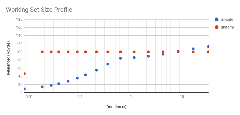
Note that I’ve used a log x-axis (here is a linear version). A sharp slope and then a flat profile is what we’d expect from a uniform distribution: the initial measurements haven’t reached its WSS as the interval is so small, and there hasn’t been enough CPU cycles to touch all the pages. As for mysqld: it takes longer to level out a little, which it does at 80 Mbytes after 16 ms, and then picks up again at 256 ms and climbs more. It looks like 80 Mbytes is hotter than the rest. Since workloads can vary second-by-second, I wouldn’t trust a single profile: I’d want to take several and plot them together, to look for the trend.

The «sharp slope» of the uniform distribution above only had one data point. Here is a 2 Gbyte WSS instead, also a uniform distribution, which takes longer for the program to reference, giving us more points to plot:

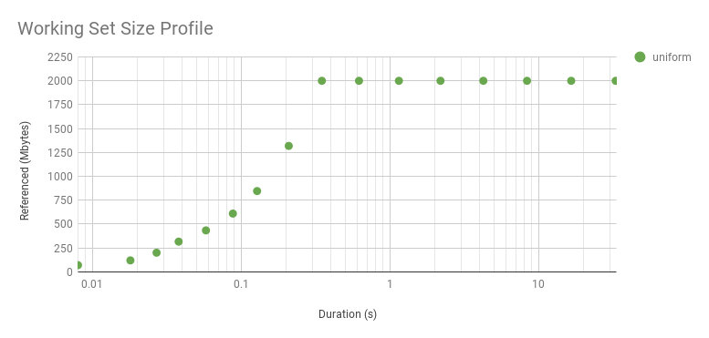
It curves upwards because it’s a log axis. Here is linear (zoomed). While it looks interesting, this curve is just reflecting the WSS sample duration rather than the access distribution. The distribution really is uniform, as seen by the flat line after about 0.3 s. The knee point in this graph shows the minimum interval we can identify a uniform access distribution, for this WSS and program logic. The profile beyond this point reflects the access distribution. The profile beyond this point reflects the access distribution, and is interesting for understanding main memory usage. The profile before it is interesting for a different reason: understanding the workload that the CPU caches process over short intervals.

6.1.7. Estimated Duration and Accuracy

Here’s how you might imagine this tool works:

1. Reset referenced page flags for a process (instantaneous)
2. Sleep for the duration
3. Read referenced page flags (instantaneous)

Here’s what really happens:

1. Reset the first page flag for a process
2. [. Reset the next page flag, then the next, then the next, etc. . ]
3. Page flag reset completes
4. Sleep for a duration
5. Read the first page flags for the process
6. [. Read the next page flag, then the next, then the next, etc. . ]
7. Read complete

The working set is only supposed to be measured during step 4, the intended duration. But the application can touch memory pages after the flag was set during step 2, and before the duration has begun in step 4. The same happens for the reads in step 6: an application may touch memory pages during this stage before the flag was checked. So steps 2 and 6 effectively inflate the sleep duration. These stages for large processes (>100 Gbytes) can take over 500 ms of CPU time, and so a 10 ms target duration can really be reflecting 100s of ms of memory changes.

To inform the end user of this duration inflation, this tool provides an estimated duration, measuring from the midpoint of stage 2 to the midpoint of stage 6. For small processes, this estimated duration will likely equal the intended duration. But for large processes, it will show the inflated time.

6.1.8. Precise Working Set Size Durations

I’ve experimented with one way to get precise durations: sending the target process SIGSTOP and SIGCONT signals, so that it is paused while page maps are set and read, and only runs for the intended duration of the measurement. This is dangerous

6.2. Experimentation: Linux Idle Page Flag

This is a newer approach added in Linux 4.3 by Vladimir Davydov, which introduces Idle and Young page flags for more reliable working set size analysis, and without drawbacks like mucking with the referenced flag which could confuse the kernel reclaim logic. Jonathan Corbet has again written about this topic: Tracking actual memory utilization. Vladimir called it idle memory tracking, not to be confused with the idle page tracking patchset from many years earlier which introduced a kstaled for page scanning and summary statistics in /sys (which was not merged).

This is still a PTE accessed-bit approach: these extra idle and young flags are only in the kernel’s extended page table entry (page_ext_flags), and are used to help the reclaim logic.

Idle memory tracking is a bit more involved to use. From the kernel documentation vm/idle_page_tracking.txt:

I’ve written two proof-of-concept tools that use this, which are in the wss collection.

6.2.1. wss-v1: small process optimized

This version of this tool walks page structures one by one, and is suited for small processes only. On large processes (>100 Gbytes), this tool can take several minutes to write. See wss-v2.c, which uses page data snapshots and is much faster for large processes (50x), as well as wss.pl, which is even faster (although uses the referenced page flag).

Here is some example output, comparing this tool to the earlier wss.pl:

The output shows that that process referenced 10 Mbytes of data (this is correct: it’s a synthetic workload).

• Est(s): Estimated WSS measurement duration: this accounts for delays with setting and reading pagemap data.
• Ref(MB): Referenced (Mbytes) during the specified duration. This is the working set size metric.

6.2.2. wss-v1 WARNINGs

This tool sets and reads process page flags, which for large processes (> 100 Gbytes) can take several minutes (use wss-v2 for those instead). During that time, this tool consumes one CPU, and the application may experience slightly higher latency (eg, 5%). Consider these overheads. Also, this is activating some new kernel code added in Linux 4.3 that you may have never executed before. As is the case for any such code, there is the risk of undiscovered kernel panics (I have no specific reason to worry, just being paranoid). Test in a lab environment for your kernel versions, and consider this experimental: use at your own risk.

6.2.3. wss-v2: large process optimized

This version of this tool takes a snapshot of the system’s idle page flags, which speeds up analysis of large processes, but not small ones. See wss-v1.c, which may be faster for small processes, as well as wss.pl, which is even faster (although uses the referenced page flag).

Here is some example output, comparing this tool to wss-v1 (which runs much slower), and the earlier wss.pl:

The output shows that that process referenced 15 Mbytes of data (this is correct: it’s a synthetic workload).

• Est(s): Estimated WSS measurement duration: this accounts for delays with setting and reading pagemap data.
• Ref(MB): Referenced (Mbytes) during the specified duration. This is the working set size metric.

6.2.4. wss-v2 WARNINGs

This tool sets and reads system and process page flags, which can take over one second of CPU time, during which application may experience slightly higher latency (eg, 5%). Consider these overheads. Also, this is activating some new kernel code added in Linux 4.3 that you may have never executed before. As is the case for any such code, there is the risk of undiscovered kernel panics (I have no specific reason to worry, just being paranoid). Test in a lab environment for your kernel versions, and consider this experimental: use at your own risk.

7. Experimentation: MMU Invalidation

This approach invalidates memory pages in the MMU, so that the MMU will soft fault on next access. This causes a load/store operation to hand control to the kernel to service the fault, at which point the kernel simply remaps the page and tracks that it was accessed. It can be done by the kernel, or the hypervisor for monitoring guest WSS.

7.2. Windows Reference Set

Microsoft have a great page on this: Reference sets and the system-wide effects on memory use. Some terminology differences:

Linux resident memory == Windows working set
Linux working set == Windows reference set

This method uses WPR or Xperf to collect a «reference set», which is a trace of accessed pages. I haven’t done these myself yet, but it appears to use the MMU invalidation approach, followed by event tracing of page faults. The documentation notes the overheads:

WARNING: «Recording the trace of a reference set can have a significant effect on system performance, because all processes must fault large numbers of pages back into their working sets after their working sets are emptied.»

I’ll update this page with more details once I’ve used it. So far these are the only tools I’ve seen (other than the ones I wrote) to do WSS estimation.

Other

Other techniques for WSS estimation include:

• Application metrics: it depends on the application, but some may already track in-use memory as a WSS approximate.
• Application modifications: I’ve seen this studied, where application code is modified to track in-use memory objects. This can add significant overhead, and requires code changes.
• CPU simulation: tracking load/stores. Apps can run 10x or more slower in such simulators.
• Memory breakpoints: such as those that debuggers can configure. I’d expect massive overhead.
• Memory watchpoint: an approach could be built to use these; watchpoints were recently supported by bpftrace.
• MMU page invalidation: forcing pages to fault on access, revealing which are in use. This could be done by the kernel, or the hypervisor for monitoring guest WSS.
• Processor trace: and similar processor-level features that can log load/stores. Expected high overhead to process the log.
• Memory bus snooping: using custom hardware physically connected to the memory bus, and software to summarize observed accesses.

What I haven’t seen is a ready-baked general purpose tool for doing WSS estimation. This is what motivated me to write my wss tools, based on Linux referenced and idle page flags, although each tool has its own caveats (although not as bad as other approaches).

Источник